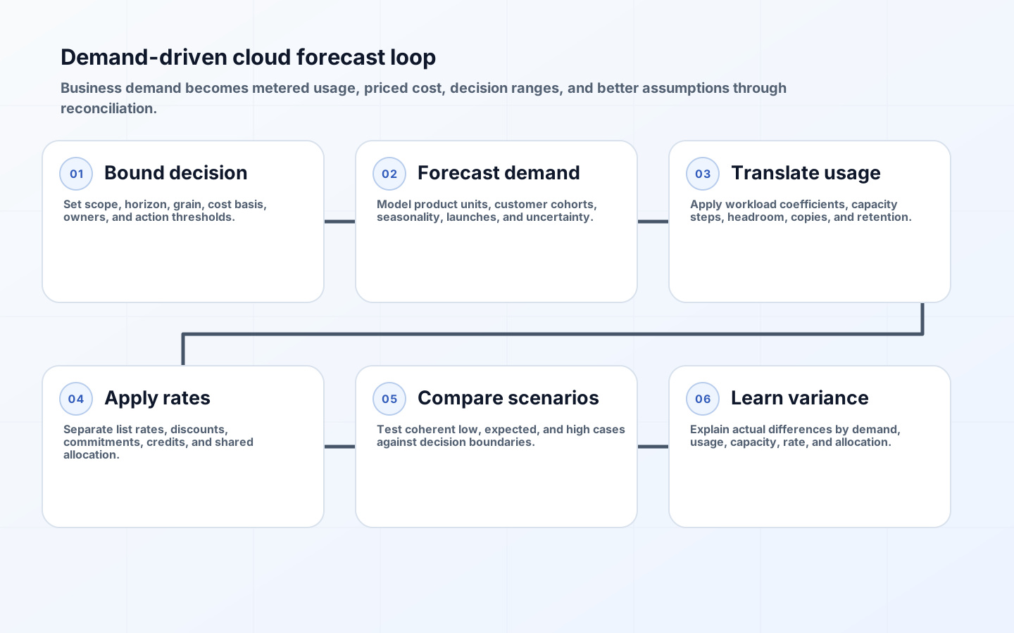
A cloud bill is a record of what happened under yesterday's product mix, architecture, traffic, prices, and operational choices. It is not a model of what will happen after a launch, a large tenant arrives, retention changes, or an efficiency project lands. Driver-based cloud cost forecasting starts with those future business events and translates them into resource usage before applying rates. The result is a forecast that product, engineering, FinOps, and finance can inspect together instead of a percentage pasted onto last month's invoice.
The goal is not false precision. It is an explainable range with named assumptions, accountable owners, and an update loop. The FinOps Framework treats estimating as exploration, forecasting as an agreed expectation, and budgeting as the allocation of funding. Keeping those jobs distinct matters: teams may compare several architectures during estimation, commit to one operating forecast, and still need a budget decision. A useful model preserves that chain and exposes why actual spend differs.
Set the forecast boundary and decision
Begin with a decision, scope, horizon, and grain. A quarterly funding decision may need monthly product-level totals, while a launch-readiness decision may need daily estimates by environment and service. Name included accounts, shared platforms, support charges, taxes, credits, and commitment treatment. Also state whether values represent list cost, billed cost, amortized cost, or an internally allocated cost. Two teams can use the same usage projection and still disagree because they silently price different cost concepts.
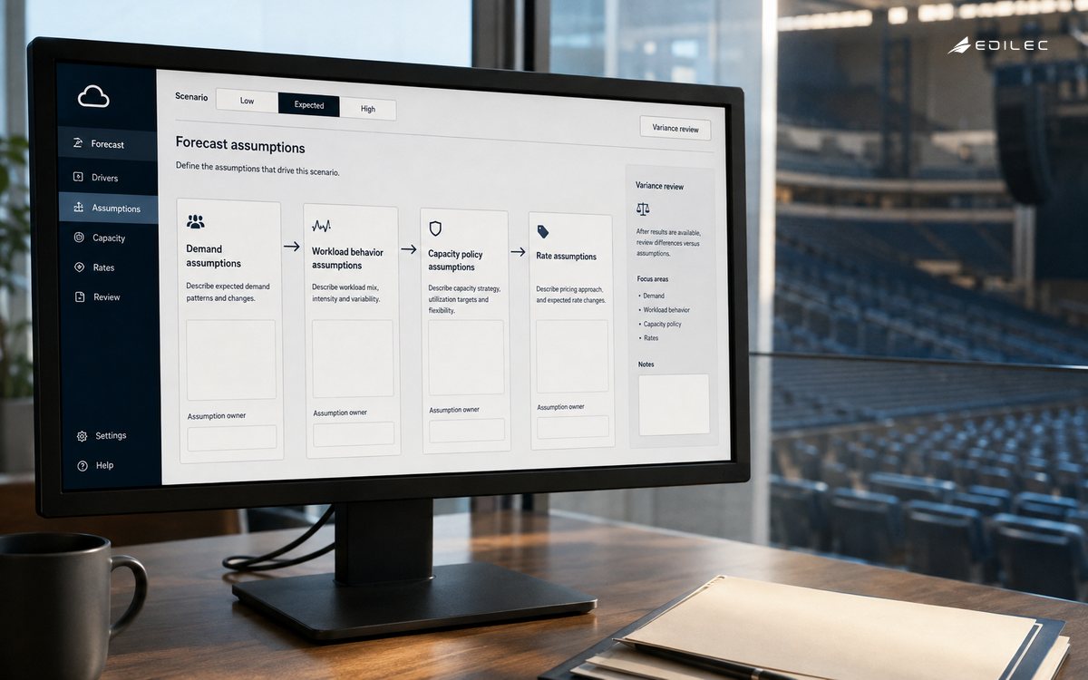
Assign one owner to the forecast baseline and one owner to each material assumption. Product owns demand events and customer mix; engineering owns workload coefficients and capacity policy; FinOps owns billing normalization, effective rates, and allocation; finance owns budget timing and reporting treatment. Ownership does not mean unilateral control. It means that a surprising value has someone who can investigate and approve a revision.
| Forecast layer | Representative input | Primary owner | Review trigger |
|---|---|---|---|
| Business demand | Active tenants, transactions, seats, uploads | Product | Launch, sales plan, churn shift |
| Workload behavior | Requests per transaction, bytes per upload | Engineering | Code or architecture change |
| Capacity policy | Headroom, replicas, retention, recovery target | Engineering and SRE | Reliability policy change |
| Price and discounts | SKU rate, tier, commitment coverage | FinOps | Contract or price change |
| Financial treatment | Allocation, amortization, currency, tax | FinOps and finance | Reporting policy change |
Model product demand as measurable events
Choose demand drivers that explain workload rather than merely correlate with the invoice. Monthly active users may predict authentication traffic but poorly explain video transcoding; uploaded minutes, output resolutions, and retry rates are stronger drivers. A B2B platform may need tenant cohorts because one enterprise customer can consume more storage and query capacity than thousands of small accounts. Prefer drivers already present in product analytics or operating systems, with stable definitions and historical coverage.
Represent known roadmap events explicitly instead of hiding them in a growth rate. Record launch date, ramp shape, eligible population, expected adoption, and uncertainty. Separate base demand, committed events, and speculative upside. For each driver, build low, expected, and high paths. Correlation among drivers also matters: transactions, bytes, and active users should not all receive independent optimistic multipliers when they describe the same growth event.
- Use a stable unit such as order, inference, streamed minute, active tenant, or gigabyte retained.
- Version the demand dataset and preserve the product plan that produced each forecast.
- Record seasonality, weekday patterns, regional rollout, and one-time migrations separately.
- Keep demand assumptions independent from cloud prices so either side can change without rebuilding the model.
Translate demand into resource usage
Build a coefficient chain from each product unit to a metered cloud quantity. An order might produce API requests, queue messages, database writes, log bytes, and downstream scans. A retained gigabyte may create primary storage, replicas, snapshots, index overhead, and network transfer. Estimate coefficients from representative telemetry, load tests, or controlled trials. Use distributions when behavior is skewed; an average tenant can conceal a small cohort that sets peak capacity.
Then apply capacity policy. Autoscaling does not make required capacity equal average demand. Minimum replicas, failover reserve, concurrency limits, burst buffers, bin-packing loss, provisioned throughput, and recovery objectives can create step functions. Model these rules directly. For example, a database tier may jump when storage or IOPS crosses a threshold, while a serverless function scales nearly continuously but introduces request and duration dimensions. These shapes are why linear bill extrapolation fails.
| Driver | Usage equation example | Important sensitivity | Validation signal |
|---|---|---|---|
| API transactions | Transactions x requests x compute-seconds | Cache hit rate and latency | Requests and billed duration |
| Customer data | New bytes x replicas x retention | Compression and deletion | Logical versus billed storage |
| Analytics queries | Queries x bytes scanned | Partition pruning | Scanned bytes per query class |
| Video minutes | Minutes x renditions x processing factor | Codec and retry rate | Compute time per output minute |
| Peak sessions | Peak concurrency / safe sessions per instance | Headroom and failover | Saturation at target latency |
Price usage without mixing rate effects
Price each metered quantity with the rate expected during the forecast period. Preserve list price, negotiated adjustments, commitment amortization, and effective rate as separate fields. Commitments can lower the rate while creating a fixed obligation, so a model should show both eligible usage and expected coverage. Credits should not erase the underlying workload cost; model their expiry independently so the forecast does not show a mysterious increase when a temporary credit ends.
Shared costs need an explicit rule. Allocate a platform cost using the causal driver when practical, such as requests, compute time, storage, or reserved capacity. Use a simple documented proxy when causal measurement costs more than the decision is worth. Always retain the unallocated total and reconcile allocated values to it. A unit-cost metric that omits shared observability, security, support, or idle capacity may look precise while moving costs outside the product boundary.
Use scenarios and sensitivity, not one magic number
Create a baseline from expected demand and current approved architecture, then vary the few assumptions that materially change the answer. Typical sensitivities include adoption, large-customer mix, data retention, cache effectiveness, model size, regional replication, purchase coverage, and delivery date. Change one variable at a time to reveal leverage, then combine coherent low and high cases. Monte Carlo simulation can help when distributions are credible, but it cannot repair invented inputs.
Attach actions to thresholds. If high-case demand consumes failover headroom, engineering may need a capacity change before launch. If unit cost exceeds margin tolerance, product can change packaging, retention, or service level. If commitment utilization falls in the low case, FinOps can delay a purchase. A forecast earns attention when its range changes a current decision; a wide range with no action boundary is merely uncertainty expressed as a chart.
Operate a variance learning loop
After each period, compare forecast and actual at every layer: business demand, workload coefficient, capacity, quantity, effective rate, and allocation. Spend variance alone cannot say whether product adoption beat plan or a logging change multiplied bytes. Store the original forecast, later revisions, actuals, and reason codes. Avoid rewriting history; forecast drift and forecast accuracy answer different questions. A revised forecast may be accurate while the original planning assumption was poor.
Set review frequency to decision speed. Fast-growing usage may need weekly driver updates and a monthly finance lock, while stable storage can be reviewed monthly. Use materiality thresholds in both currency and percentage terms because a large percentage on a tiny service and a small percentage on a major platform imply different work. Recalibrate coefficients when error persists, not whenever one noisy week misses the line.
Implement the model as a governed data product
Start with one product whose bill is material and whose demand telemetry is credible. Build a versioned input table, coefficient table, price table, calculation model, and reconciliation output. Test dimensional units so bytes, gigabytes, seconds, hours, and currencies cannot silently mix. Back-test several past periods using only information that would have been available then. Publish assumptions beside results and restrict manual overrides to named fields with an owner and expiry.
Do not wait for perfect allocation. Expose an explicit residual and improve it as decisions require. Automate ingestion only after definitions stabilize; otherwise the pipeline makes changing semantics appear authoritative. A mature implementation can feed budgets and alerts, but it should retain a human sign-off for roadmap events and unusual pricing. The operating control is traceability from forecast total back to demand, quantity, rate, and responsible assumption.
Key takeaways
- Forecast product demand first, translate it into metered usage, and price that usage separately.
- Model capacity steps, reliability reserve, shared cost, credits, and commitments rather than assuming linear growth.
- Use scenarios with action thresholds so uncertainty informs a present decision.
- Decompose variance by demand, workload, capacity, rate, and allocation to improve the model.
- Keep every forecast version, assumption owner, and reconciliation result auditable.
Frequently asked questions
Should historical spend be discarded?
No. Historical cost and usage are essential for calibration, back-testing, seasonality, and anomaly detection. They should constrain the driver model rather than substitute for it. When history and the modeled future disagree, identify the product, architecture, capacity, or price event that explains the break.
What accuracy target is reasonable?
Set targets by horizon, scope, and decision. Near-term product totals should normally be tighter than a new service six months away. Use percentage and absolute variance, track bias, and judge whether errors cross funding or capacity thresholds. One universal accuracy percentage encourages gaming and hides material differences.
Which unit cost should a team use?
Choose a unit tied to customer or business value and sufficiently causal for technology use. Orders, active tenants, documents processed, or streamed hours are often stronger than raw requests. Publish the cost boundary and denominator definition so changes in product mix do not masquerade as efficiency.
Conclusion
Driver-based cloud cost forecasting turns a financial total into an operational explanation. By linking product demand to workload coefficients, capacity policy, metered quantities, rates, and allocation, teams can see which assumption changes the outcome and who can act. The model will never remove uncertainty, but a versioned range with explicit decisions and a disciplined variance loop is far more useful than extending the latest bill into a future the product team already knows will be different.